This GSEB Class 12 Commerce Statistics Notes Part 1 Chapter 3 Linear Regression Posting covers all the important topics and concepts as mentioned in the chapter.
Linear Regression Class 12 GSEB Notes
Linear Regression Model:
- Independent Variable: Out of two variables having cause-effect relationship, the causal variable is called independent variable. It is denoted by X.
- Dependent Variable: Out of two variables having cause-effect relationship, the effect variable is called dependent variable. It is denoted by Y.
- Regression : A functional relationship between two correlated variable is called regression.
To study the regression an axiomatic assumption that there is cause-effect relation between two variables is taken.
The literal meaning of regression is ‘to avert’ or ‘return to the mean value’.
Linear Regression Model:
A regression model expressing the dependent variable Y as a linear function of independent variable X is called a Linear regression model. It is of the following form :
Y = α + βx + u
Where, Y = Dependent variable
X = Independent variable α,
β = Constants
u = Disturbance variable of model
Variable u shows the incompletness of Linear correlation between two variables X and Y.
- If there is perfect linear correlation between two variables X and Y, then the linear regression model is of the form
Y = α + β X. In such case the value of disturbance variable u will be 0 (zero). - If there is partial linear correlation between two variables X and Y, the form of linear regression- model is
Y = α +βx + u.
![]()
Fitting of Regression Line :
A method to obtain the regression line that gives the best estimated relation between two correlated variables is called fitting of regression line.
There are two methods of fitting regression line :
1. Scatter Diagram Method: This method of fitting a regression line is simple and speedy. It is subjective method and does not guarantee the best estimates
of the dependent variable. Hence, the least square method is used to obtain a best fitted regression line.
2. Least Squares Method: If the equation of best fitted regression line of Y on X is ŷ = a + bx, then the values of constants a and b are obtained by method of least square such that the sum of squares of errors Σei2 becomes least. Here, ei = yi – ŷi and ŷi = a + bxi. So, Σei2 = Σ(yi – a – bxi)
- Coefficient of Regression: The estimated change in the values of dependent variable Y due to a unit change in the value of independent variable X is called the regression coefficient of Y on X. It is denoted by ‘b’ or ‘byx’
- In y = a + bx, a = Intercept of regression line and b = slope of the regression line.
- Interpretation of regression coefficient ‘b’: → b = The estimated change in the value of Y for a unit change in the value of X.
- If b > 0: A unit increase in the value of X implies an estimated increase of b units in the value of Y. b < 0 : A unit increase in the value of X implies an estimated decrease of b units in the value of Y.
- When all points in a scatter diagram are on one line only then the form of regression line will be y = a + bx. In this case, if b > 0 then the value of r = 1 and if b < 0 the value of r = -1.
Utility of the Study of Regression:
- We can know the functional relationship between two correlated variables.
- We can estimate the unknown value of Y, for a given value of independent value of X.
- We can find the estimated change in Y, per unit change in X with the help of regression.
- We can determine the error occur in finding the estimated value of dependent variable by using the regression line.
- It is useful for economists, planners, businessmen, administrators, researchers, etc.
Coefficient of Regression from Covariance, Variance and Correlation Coefficient:
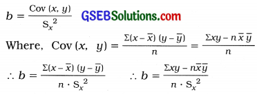
1. Covariance (x, y) and variance Sx2 are known :
b or byx = \(\frac{{Cov}(x, y)}{\mathrm{S}_{x}^{2}}\)
2. Variance Sx2, variance Sy2 of correlation r are known:
b or byx = r\(\frac{\mathrm{S}_{y}}{\mathrm{~S}_{x}}\)
Coefficient of Determination:
The square of correlation coefficient between the observed value y of the dependent variable Y and
the corresponding estimated value y of Y by the regression line y = a + bx is called the coefficient of determination. It is denoted by R2.
Thus, R2 = [Cor (y, ŷ)]2
= [Cor (y, a + bx)]2
= [Cor (y, x)]2
- If R2 = 1, estimates obtained on the basis of regression line are 100% reliable. There is perfect linear correlation between the variable Y and X.
- If R2 = 0 estimates obtained on the basis of regression line are not reliable. There is lack of linear correlation between the variables Y and X.
- If R2 is near to 1 (i.e., 0.5 ≤ R2 < 1), then the assumption of linear regression is said to be proper and estimates obtained by regression line are reliable,
- If R2 is near to ‘0’ (i.e., 0 ≤ R2 < 0.5), then the assumption of linear regression is said to be improper and the estimates obtained by regression line are not reliable.
Properties of Coefficient of Regression:
- The signs of correlation coefficient r and regression coefficient b are same.
- Value of regression coefficient b is’ independent of change of origin but not of scale.
- From regression coefficient the estimated change in the value of Y, per unit change in the value of X can be known.
- The value of b can be less than 1 or greater than 1.
- The regression coefficient is a relative measure.
- Sign of ‘b’ depends on the sign of Cov(x, y).
- If b > 0, a unit increase in X implies an estimated increase of b units in Y.
- If b < 0, a unit increase in X, implies an estimated decrease of b units in Y.
Precautions While Using Regression:
- We should make the use of the estimates obtained only after examining the assumption of linear regression by coefficient of determination R2.
- The regression relation obtained by the scatter diagram or by the least squares should not be used for the values which are very far from the given values of independent variable.
![]()
Important Formulae:
Equation of regression line of Y on X:
ŷ = a + bx Where, b = byx
= Regression coefficient of Y on X
= Slop of regression line of Y on X
a = Intercept of regression line of Y on X
1. Values of X and Y are small:
b = \(\frac{n \Sigma x y-(\Sigma x)(\Sigma y)}{n \Sigma x^{2}-(\Sigma x)^{2}}\)
2. Values of x and y are integers:
b = \(\frac{\Sigma(x-\bar{x})(y-\bar{y})}{\Sigma(x-\bar{x})^{2}}\)
3. Values of x and y are not integers (short¬cut method):
b = \(\frac{n \Sigma u v-(\Sigma u)(\Sigma v)}{n \Sigma u^{2}-(\Sigma u)^{2}}\)
Where, u = x – A and v = y – B
4. Origin and scale both are changed:
b = \(\frac{n \Sigma u v-(\Sigma u)(\Sigma v)}{n \Sigma u^{2}-(\Sigma u)^{2}} \times \frac{\mathrm{C}_{y}}{\mathrm{C}_{x}}\)
Where, u = \(\frac{x-\mathrm{A}}{\mathrm{C}_{\chi}}\) and v = \(\frac{y-\mathrm{B}}{\mathrm{C}_{y}}\),
A, B, Cx, Cy are constants.
Cx > 0, Cy > 0
5. Covariance and variance are known:

6. Correlation coefficient r, standard deviations of X and Y are known:
b = r \(\frac{\mathrm{S}_{y}}{\mathrm{~S}_{x}}\)
7. Constant a:
a = y – bx
Where, x = \(\frac{\Sigma x}{n}\) and u = \(\frac{\Sigma y}{n}\)
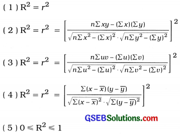
8. Coefficient of determination:
R2 = [r (y, ŷ)]2 = [r (x, ŷ)]2 = r2
