Gujarat Board Statistics Class 11 GSEB Solutions Chapter 5 Skewness of Frequency Distribution Ex 5.1 Textbook Exercise Questions and Answers.
Gujarat Board Textbook Solutions Class 11 Statistics Chapter 5 Skewness of Frequency Distribution Ex 5.1
Question 1.
The following distribution shows demand of 500 ml pouches of pasteurized toned milk by 59 consumers. Find Karl Pearson’s coefficient of skewness from these data.

Answer:
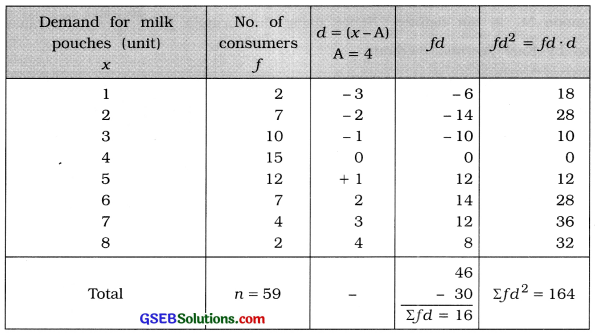
Mean:
x̄ = A + \(\frac{\Sigma f d}{n}\)
= 4 + \(\frac{16}{59}\)
= 4 + 0.27
= 4.27 pouches
Mode:
M0 = observation having maximum frequency 15
∴ M0 = 4 pouches
Standard deviation:
s = \(\sqrt{\frac{\Sigma f d^{2}}{n}-\left(\frac{\Sigma f d}{n}\right)^{2}}\)
= \(\sqrt{\frac{164}{59}-\left(\frac{16}{59}\right)^{2}}\)
= \(\sqrt{2.78-(0.27)^{2}}\)
= \(\sqrt{2.78-0.0729}\)
= \(\sqrt{2.7071}=\) = 1.65 pouches
Karl Pearson’s coefficient of skewness:
j = \(\frac{\bar{x}-\mathrm{M}_{0}}{s}\)
Putting x̄ = 4.27, M0 = 4 and s = 1.65
j = \(\frac{4.27-4}{1.65}=\frac{0.27}{1.65}\) = 0.16
Question 2.
The following distribution shows purchase of T-shirts by 270 customers according to the shoulder lengths (in inches). Find Karl Pearson’s coefficient of skewness from these data and interpret it.

Answer:
In the given frequency distribution maximum frequency 56 appears against two observation.
Therefore mode M0 is not defined. Hence using the formula j = \(\frac{3(\bar{x}-\mathrm{M})}{s}\), we calculate coefficient of skewness by Karl Pearson method.
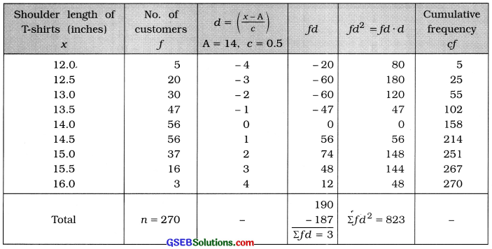
Mean:
x̄ = A + \(\frac{\Sigma f d}{n}\) × c
= 14 + \(\frac{3}{270}\) × 0.5
= 14 + \(\frac{1.5}{270}\)
= 14 + 0.01
= 14.01 inch
Median:
M = value of \(\left(\frac{n+1}{2}\right)\)th observation
= value of \(\left(\frac{270+1}{2}\right)\)th observation
= value of 135.5th observation
Referring to column cf,
M – 14 Inch
Standard Deviation:
s = \(\sqrt{\frac{\Sigma f d^{2}}{n}-\left(\frac{\Sigma f d}{n}\right)^{2}}\) × c
= \(\sqrt{\frac{823}{270}-\left(\frac{3}{270}\right)^{2}}\) × 0.5
= \(\sqrt{3.0481-(0.01)^{2}}\) × 0.5
= \(\sqrt{3.0481-0.0001}\) × 0.5
= \(\sqrt{3.048}\) × 0.5
= 1.746 × 0.5 = 0.873 ≈ 0.87 inch
Coefficient of skewness by Karl Pearson method:
j = \(\frac{3(\bar{x}-\mathrm{M})}{s}\)
= \(\frac{3(14.01-14)}{0.87}=\frac{3(0.01)}{0.87}=\frac{0.03}{0.87}\) = 0.03
Interpretation :J = 0.03. Therefore, the frequency distribution is slightly positive skewed, i.e., the measures mean and mode of length of shoulder of T-shirts are approximately same.
![]()
Question 3.
The following information is obtained for the time taken (in completed minutes) by each workers to carry out a certain job. Find Karl Pearson’s coefficient of skewness from these data and interpret it.

Answer:
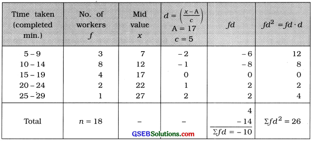
Mean:
x̄ = A + \(\frac{\Sigma f d}{n}\) × c
= 17 – \(\frac{10}{18}\) × 5
= 17 – \(\frac{50}{18}\)
= 17 – 2.78
= 14.22 minutes
Mode:
M0 class = class having maximum frequency 8
= 10 – 14
In exclusive form. M0 class = 9.5 – 14.5
Now. M0 = L + \(\frac{f_{m}-f_{1}}{2 f_{m}-f_{1}-f_{2}}\) × c
Putting L = 9.5, fm =8’ f1 = 3. f2 = 4 and c = 5 in the formula.
M0 = 9.5 + \(\frac{8-3}{2(8)-3-4}\) × 5
= 9.5 + \(\frac{5 \times 5}{16-7}\)
= 9.5 + \(\frac{25}{9}\)
= 9.5 + 2.78
= 12.28 mInutes
Standard Deviation:
s = \(\sqrt{\frac{\Sigma f d^{2}}{n}-\left(\frac{\Sigma f d}{n}\right)^{2}}\) × c
= \(\sqrt{\frac{26}{18}-\left(\frac{-10}{18}\right)^{2}}\) × 5
= \(\sqrt{1.44-(0.55)^{2}}\) × 5
= \(\sqrt{1.44-0.3025}\) × 5
= \(\sqrt{1.1375}\) × 5
= 1.0665 × 5 = 5.33 minutes
Coefficient of skewness by Karl Pearson Method :
j = \(\frac{\bar{x}-\mathrm{M}_{0}}{s}\)
Putting x̄ = 14.22, M0 = 12.28 and s = 5.33 in the formula,
j = \(\frac{14.22-12.28}{5.33}=\frac{1.94}{5.33}\) = 0.36
Interpretation : j = 0.36. Therefore, the average time taken by a worker to complete one type of work there is positive difference between mean and mode. i.e.. the frequency distribution is positively skewed.
Question 4.
The students of standard 11 have collected the data about profits (in croie ) of IT companies. Find Karl Pearson’s coefficient of skewness from these data and interpret It.

Answer:
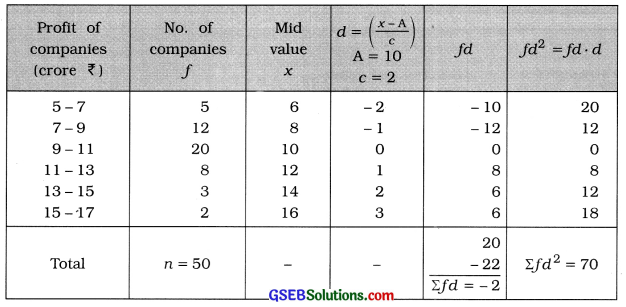
Mean:
x̄ = A + \(\frac{\Sigma f d}{n}\) × c
= 10 – \(\frac{2}{50}\) × 2
= 17 – \(\frac{4}{50}\)
= 10 – 0.008
= ₹ 9.92 crore
Mode:
M0 class = class having maximum frequency 8
= 9 – 11
Now. M0= L + \(\frac{f_{m}-f_{1}}{2 f_{m}-f_{1}-f_{2}}\) × c
Putting L =9, fm =20’ f1 = 12. f2 = 8 and c = 2 in the formula.
M0 = 9 + \(\frac{20-12}{2(20)-12-8}\) × 2
= 9 + \(\frac{8 \times 2}{40-20}\)
= 9 + \(\frac{16}{20}\)
= 9 + 0.8
= ₹ 9.8 crore
Standard Deviation:
s = \(\sqrt{\frac{\Sigma f d^{2}}{n}-\left(\frac{\Sigma f d}{n}\right)^{2}}\) × c
= \(\sqrt{\frac{70}{50}-\left(\frac{-2}{50}\right)^{2}}\) × 2
= \(\sqrt{1.4-(-0.04)^{2}}\) × 2
= \(\sqrt{1.4-0.0016}\) × 2
= \(\sqrt{1.3984}\) × 2
= 1.1825 × 2 = ₹ 2.37 crore
Coefficient of skewness by Karl Pearson Method :
j = \(\frac{\bar{x}-\mathrm{M}_{0}}{s}\)
Putting x̄ = 9.92, M0 = 9.8 and s = 2.37 in the formula,
j = \(\frac{9.92-9.8}{2.37}=\frac{0.12}{2.37}\) = 0.05
Interpretation: J = 0.05. Therefore, the distribution is slightly positive skewed. i.e.. the mean and mode of profit of IT companies are approximately same.
![]()
Question 5.
The following frequency distribution gives the amount of annual depreciation (in lakh ₹) of 38 companies. Using this information, find skewness and its coefficient by Karl Pearson’s method. State the type of skewness.

Answer:
The frequency distribution of the given data is combined type. Therefore mode is not defined.
Hence, using Sk = 3 (x – M) and we calculate skewness and coefficient the formula j = \(\frac{3(\bar{x}-\mathrm{M})}{s}\) of skewness.
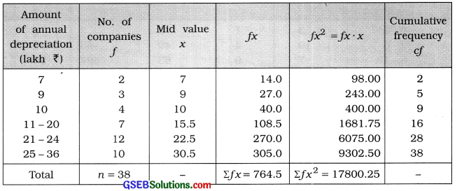
Mean:
x̄ = \(\frac{\Sigma f x}{n}=\frac{764.5}{38}\)
= ₹ 20.12 lakh
Median:
M class = class that Includes \(\left(\frac{n}{2}\right)\)th observation
= class that includes \(\left(\frac{38}{2}\right)\)th observation
= class that includes 19th observation
Referring to column cf.
M class = 21 – 24
In exclusive form. M class = 20.5 – 24.5
Now. M = L + \(\frac{\frac{n}{2}-c f}{f}\) × c
Putting L = 20.5. \(\frac{n}{2}\) = 19. cf = 16. f = 12 and c = 4 in the formula.
M = 20.5 + \(\frac{19-16}{12}\) × 4
= 20.5 + \(\frac{3 \times 4}{12}\)
= 20.5 + 1
= ₹ 21.5 lakh
Standard Deviation:
s = \(\sqrt{\frac{\Sigma f x^{2}}{n}-\left(\frac{\Sigma f x}{n}\right)^{2}}\)
= \(\sqrt{\frac{17800.25}{38}-\left(\frac{764.5}{38}\right)^{2}}\)
= \(\sqrt{468.43-(20.12)^{2}}\)
= \(\sqrt{468.43-404.81}\)
= \(\sqrt{63.62}\)
= ₹ 7.98 lakh
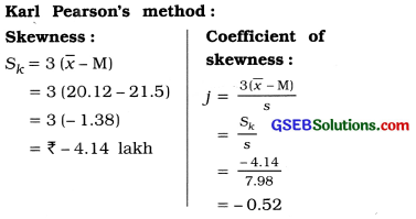
Type of skewness:
Sk = – 4.14. Therefore, the given frequency distribution Is negatively skewed.
Question 6.
The monthly consumption of cotton (in thousand bales) of 35 cloth mills is as follows. Using this, find skewness and its coefficient by Karl Pearson’s method. State the type of skewness.

Answer:
The given frequency distribution is of unequal length. Therefore mode is not defined. Hence, using the formulae Sk = 3 (x̄ – M) and j = \(\frac{3(\bar{x}-\mathrm{M})}{s}\) we will find skewness and coefficient of skewness.
Mean:
x̄ = \(\frac{\Sigma f x}{n}=\frac{361}{35}\)
= 10.31 thousand bales
Median:
M class = class that Includes \(\left(\frac{n}{2}\right)\)th observation
= class that includes \(\left(\frac{35}{2}\right)\)th observation
= class that includes 17.5th observation
Referring to column cf. M class = 6 – 12
Now. M = L + \(\frac{\frac{n}{2}-c f}{f}\) × c
Putting L = 6. \(\frac{n}{2}\) = 17.5. cf = 13. f = 7 and c = 6 in the formula.
M = 6 + \(\frac{17.5-13}{7}\) × 6
= 6 + \(\frac{4.5 \times 6}{7}\)
= 6 + 3.86
= 9.86 thousand bales
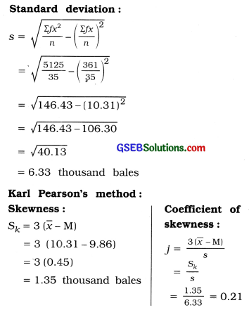
Type of skewness:
j = 0.21. Therefore, the given frequency distribution is positively skewed.
![]()
Question 7.
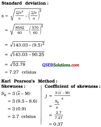
The temperature (in Celsius) at a tourist place for 60 days in the year 2014 is as follows. Using this information, find skewness and its coefficient by Karl Pearson’s method. State the type of skewness.

Answer:
The given frequency distribution is of unequal class length. Therefore mode is not defined. Using the formulae Sk = 3 (x – M) and j = \(\frac{3(\bar{x}-\mathrm{M})}{\mathrm{s}}\) we will find skewness and coefficient of skewness.
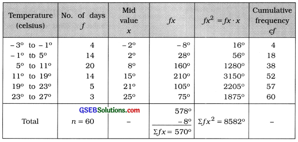
Mean:
x̄ = \(\frac{\Sigma f x}{n}=\frac{361}{35}\)
= 10.31 thousand bales
Median:
M class = class that Includes \(\left(\frac{n}{2}\right)\)th observation
= class that includes \(\left(\frac{60}{2}\right)\)th observation
= class that includes 30th observation
Referring to column cf. M class = 5° to 11°
Now. M = L + \(\frac{\frac{n}{2}-c f}{f}\) × c
Putting L = 5. \(\frac{n}{2}\) = 30. cf = 18. f = 20 and c = 6 in the formula.
M = 5 + \(\frac{30-18}{20}\) × 6
= 5 + \(\frac{12 \times 6}{20}\)
= 5 + \(\frac{72}{20}\)
= 5 + 3.6
= 8.6 celsius
Type of skewness:
j = 0.37. Therefore, the given frequency distribution is positively skewed.