Gujarat Board Statistics Class 12 GSEB Solutions Part 1 Chapter 3 Linear Regression Ex 3.2 Textbook Exercise Questions and Answers.
Gujarat Board Textbook Solutions Class 12 Statistics Part 1 Chapter 3 Linear Regression Ex 3.2
Question 1.
The following information is obtained from a study to know the effect of use of fertilizer on the yield of cotton:
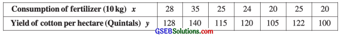
Obtain the regression line of Y on X and estimate the yield of cotton per hectare if 300 kg fertilizer is used.
Answer:
Here, n = 7; X = Consumption of fertilizer and Y = Yield of cotton.
Now, x̄ = \(\frac{\Sigma x}{n}\) = \(\frac{177}{7}\) = 25.29; ȳ = \(\frac{\Sigma y}{n}\) = \(\frac{830}{7}\) = 118.57
We obtain the regression line of yield of cotton (Y) on the consumption of fertilizer (X) ŷ = a + bx.
x̄ and ȳ are not integers. So we calculate ‘a’ and ‘b’ by shortcut method taking new variables
u = x – A, A = 25 and v = y – B, B = 120.
The table for calculation is prepared as follows:
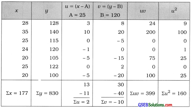
b = \(\frac{n \Sigma u v-(\Sigma u)(\Sigma v)}{n \Sigma u^{2}-(\Sigma u)^{2}}\)
Putting n = 7; Σuv = 399; Σu = 2; Σv = – 10 and Σu2 =160 in the formula,
b = \(\frac{7(399)-(2)(-10)}{7(160)-(2)^{2}}\)
= \(\frac{2793+20}{1120-4}\)
= \(\frac{2813}{1116}\)
= 2.52
a = ȳ – bx̄
Putting ȳ = 118.57; x̄ = 25.29 and b = 2.52, we get
a = 118.57 – 2.52 (25.29)
= 118.57 – 63.73
= 54.84
Regression line of Y on X:
Putting a = 54.84 and b = 2.52 in ŷ = a + bx, we get
ŷ = 54.84 + 2.52
Estimate of Y when X = 30 :
Putting x = 30 in ŷ = 54.84 + 2.52 x, we get
ŷ = 54.84 + 2.52 (30)
= 54.84 + 75.6
= 130.44
Hence, the estimate of Y obtained is ŷ 130.44 Quintals.

Question 2.
To know the relationship between the heights of father and sons, obtain the regression line of height of son on the height of father from the following information of eight pairs of fathers and adult sons.
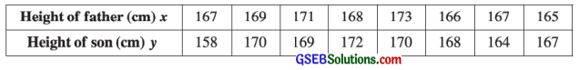
Estimate the height of a son whose father’s height is 170 cm.
Answer:
Here, n = 8; X = Height of father and Y = Height of son
Now, x̄ = \(\frac{\Sigma x}{n}\) = \(\frac{1346}{8}\) = 168.25 cm; ȳ = \(\frac{\Sigma y}{n}\) = \(\frac{1338}{8}\) = 167.25 cm
We obtain the regression line of height of son (Y) on height of father (Y) ŷ = a + bx.
x̄ and ȳ are not integers. So we calculate the values of a and b by shortcut method taking new variables
u = x – A, A = 168 and v = y – B, B = 167.
The table for calculation is prepared as follows:
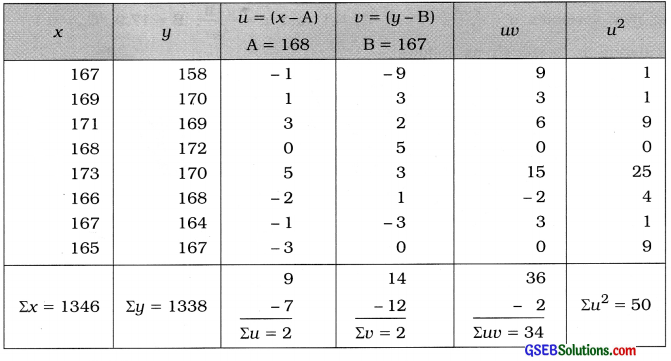
b = \(\frac{n \Sigma u v-(\Sigma u)(\Sigma v)}{n \Sigma u^{2}-(\Sigma u)^{2}}\)
Putting n = 8; Σuv = 34; Σu = 2; Σv = 2 and Σu2 = 50 in the formula,
b = \(\frac{8(34)-(2)(2)}{8(50)-(2)^{2}}\)
= \(\frac{272-4}{400-4}\)
= \(\frac{268}{396}\)
= 0.68
a = ȳ – bx̄
Putting ȳ = 167.25; x̄ = 168.25 and b = 0.68, we get
a = 167.25 – 0.68 (168.25)
= 167.25 – 114.41
= 52.84
Regression line of Y on X:
Putting a = 52.84 and b = 0.68 in ŷ = a + bx, we get
ŷ = 52.84 + 0.68x
Estimate of Y when X = 170 cm:
Putting x = 170 in ŷ = 52.84 + 0.68 x, we get
ŷ = 52.84 + 0.68 (170)
= 52.84 + 115.6
= 168.44
Hence, the estimate of son height obtained is ŷ = 168.44 cm.
Question 3.
From the following information of altitude and the amount of effective oxygen in air at the place, obtain the regression line of amount of effective oxygen (Y) on the altitude (X): (305 metre = 1000 feet)
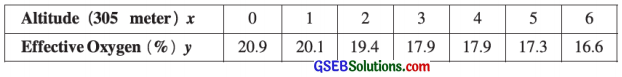
If the altitude of a place is 7 units (1 unit = 305 metre), estimate the percentage of effective oxygen in air at that place.
Answer:
Here, n = 7; X = Altitude and Y = Effective oxygen
Now, x̄ = \(\frac{\Sigma x}{n}\) = \(\frac{21}{7}\) = 3; ȳ = \(\frac{\Sigma y}{n}\) = \(\frac{130.1}{7}\) = 18.59
We obtain the regression line of effective oxygen (Y) on altitude (X) ŷ = a + bx.
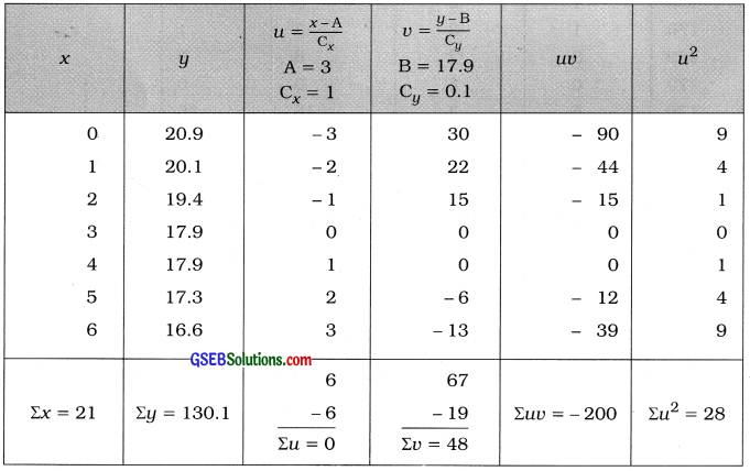
ŷ is not integer and its values are multiple of 0.1. We calculate the values of a and b by short-cut method taking new variables
u = \(\frac{x-\mathrm{A}}{\mathrm{C}_{x}}\); A = 3, Cx = 1 and v = \(\frac{y-B}{C_{y}}\); B = 17.9, Cy = 0.1.
The table for calculation is prepared as follows:
b = buv = \(\frac{n \Sigma u v-(\Sigma u)(\Sigma v)}{n \Sigma u^{2}-(\Sigma u)^{2}} \times \frac{\mathrm{C}_{y}}{\mathrm{C}_{x}}\)
Putting n = 7; Σuv = – 200; Σu = 0; Σu = 48; Σu2 = 28; Cy = 0.1 and Cx = 1 in the formula,
b = \(\frac{7(-200)-(0)(48)}{7(28)-(0)^{2}} \times \frac{0.1}{1}\)
= \(\frac{-1400-0}{196-0} \times \frac{0.1}{1}\)
= \(\frac{-1400 \times 0.1}{196}\)
= \(\frac{-140}{196}\)
= – 0.71
a = ȳ – bx̄
Putting ȳ = 18.59; x̄ = 3 and b = – 0.71, we get
a = 18.59 – (- 0.71) (3)
= 18.59 + 2.13
= 20.72
The regression line og Y on X:
Putting a = 20.72 and b = – 0.71, we get ŷ = 20.72 – 0.71x
The estimate of percentage of oxygen (Y) when X = 7:
Putting x = 7 in y = 20.72 – 0.7 lx, we get
ŷ = 20.72 – 0.71 (7)
= 20.72 – 4.97
= 15.75
Hence, the estimate of percentage of oxygen obtained is ŷ = 15.75%.
Question 4.
The following information is obtained to study the relation between the carpet area in a house and its monthly rent in a city:
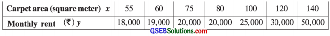
Obtain the regression line of Y on X. Estimate the monthly rent of a house having carpet area of 110 square metre.
Answer:
Here, n = 7; X = Carpet area and Y = Monthly rent.
Now, x̄ = \(\frac{\Sigma x}{n}\) = \(\frac{630}{7}\) = 90; ȳ = \(\frac{\Sigma y}{n}\) = \(\frac{182000}{7}\) = 26000
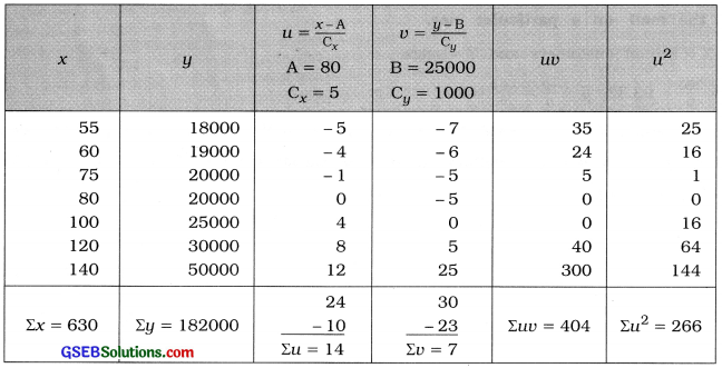
To obtain the regression line ŷ = a + bx of monthly rent (Y) on the carpet area (X), we calculate
the values of a and b by shortcut method, taking new variables u = \(\frac{x-\mathrm{A}}{\mathrm{C}_{x}}\), A = 80, Cx = 5 and v = \(\frac{y-\mathrm{B}}{\mathrm{C}_{y}}\), B = 25000, Cy = 1000
The table for calculation is prepared as follows:
b = bvu = \(\frac{n \Sigma u v-(\Sigma u)(\Sigma v)}{n \Sigma u^{2}-(\Sigma u)^{2}} \times \frac{\mathrm{C}_{y}}{\mathrm{C}_{x}}\)
Putting n = 7; Σuv = 404; Σu = 14; Σv = 7; Σu2 = 266; Cx = 5 and Cy = 1000 in the formula,
b = \(\frac{7(404)-(14)(7)}{7(266)-(14)^{2}} \times \frac{1000}{5}\)
= \(\frac{2828-98}{1862-196}\) × 200
= \(\frac{2730 \times 200}{1666}\)
= \(\frac{546000}{1666}\)
= 327.73
a = ȳ – bx̄
Putting ȳ = 26000; b = 327.73 and x̄ = 90, we get
a = 26000 – 327.73 (90)
= 26000 – 29495.7
= – 3495.7
Regression line of Y on X:
Putting a = – 3495.7 and b = 327.73 in ŷ = a + bx, we get
ŷ = – 3495.7 + 327.73x
Estimate of monthly rent (Y) when X=110:
Putting x = 110 in ŷ = – 3495.7 + 327.73x, we get
ŷ = – 3495.7 + 327.73 (110)
= – 3495.7 + 36050.3
= 32554.6
Hence, the estimate of monthly rate obtained is ŷ = ₹ 32554.6
Question 5.
The following sample data is obtained to study the relation between the number of customers visiting a mall per day and the sales (ten thousand ₹) :
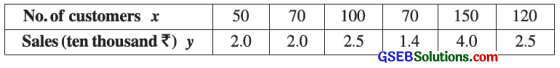
Obtain the regression line of Y on X. Estimate the sales of a mall if 80 customers have visited the mall on a particular day.
Answer:
Here, n = 6; X = No. of customers and Y = sales.
Now, x̄ = \(\frac{\Sigma x}{n}\) = \(\frac{560}{6}\) = 93.33; ȳ = \(\frac{\Sigma y}{n}\) = \(\frac{14.4}{6}\) = 2.4
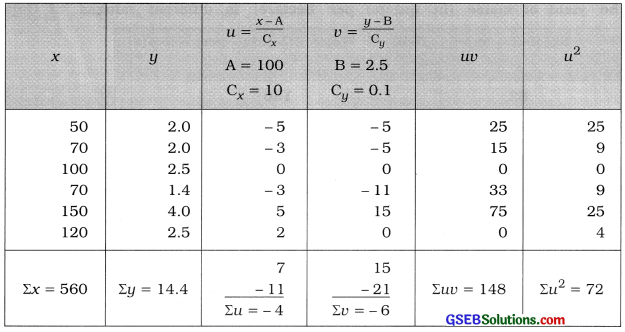
To obtain tire regression line ŷ = a + bx of sales (Y) on the number of customers (X), we calculate the values of a and b by shortcut method, taking new variables u = \(\frac{x-\mathrm{A}}{\mathrm{C}_{x}}\), A = 100, Cx = 10 and v = \(\frac{y-\mathrm{B}}{\mathrm{C}_{y}}\), B = 2.5, Cy = 0.1.
The table for calculation is prepared as follows:
b = \(\frac{n \Sigma u v-(\Sigma u)(\Sigma v)}{n \Sigma u^{2}-(\Sigma u)^{2}} \times \frac{\mathrm{C}_{y}}{\mathrm{C}_{x}}\)
Putting n = 6; Σuv = 148; Σu = – 4; Σv = – 6;
Σu2 = 72; Cx = 10 and Cy = 0.1 in the formula.
b = \(\frac{6(148)-(-4)(-6)}{6(72)-(-4)^{2}} \times \frac{0.1}{10}\)
= \(\frac{888-24}{432-16} \times \frac{0.1}{10}\)
= \(\frac{864 \times 0.1}{416 \times 10}\)
= \(\frac{86.4}{4160}\)
= 0.02
a = ȳ – bx̄
Putting ȳ = 2.4; x̄ = 93.33 and b = 0.02, we get
a = 2.4 – 0.02 (93.33)
= 2.4- 1.87
= 0.53
Regression line of Y on X:
Putting a = 0.53 and b = 0.02 in ŷ = a + bx,
we get ŷ = 0.53 + 0.02x
Estimate of sales Y when X = 80 :
Putting x = 80 in ŷ = 0.53 + 0.02x, we get
ŷ = 0.53 + 0.02 (80)
= 0.53 + 1.6 = 2.13
Hence, the estimate of sales obtained is ŷ = ₹ 2.13 (ten thousand).
Question 6.
The following information is given for ten firms running business of clothes in a city regarding their average annual profit (in lakh ₹) and average annual administrative cost (in lakh ₹) :
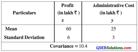
Answer:
Here, x̄ = 60; ȳ = 25; Sx = 6; Sy = 3 and Cov (x, y) = 10.4
Regression line of Y on X:
ŷ = a + bx
b = \(\frac{{Cov}(x, y)}{{S}_{x}^{2}}\)
= \(\frac{10.4}{(6)^{2}}\)
= \(\frac{10.4}{36}\)
= 0.29
a = ȳ – bx̄
= 25 – 0.29(60)
= 25 – 17.4
= 7.6
Putting a = 7.6 and b = 0.29 in ŷ = a + bx, we get ŷ = 7.6 + 0.29 x
Question 7.
The following information is obtained to study the relationship between average rainfall (in cm) and the yield of maize (in quintal per hectare) in different talukaa of Gujarat:
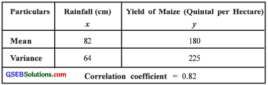
Estimate the yield of maize when the rainfall is 60 cm.
Answer:
Here, x̄ = 82; ȳ = 180; r = 0.82; Sx2 = 64
∴ Sx = 8 and Sy2 = 225
∴ Sy = 15 are given.
To estimate the yield of maize (Y) when the rainfall (X) is 60 cm we obtain the regression line of Y on X, ŷ = a + bx.
Now, b = r ∙ \(\frac{\mathrm{S}_{y}}{\mathrm{~S}_{x}}\);
Putting r = 0.82; Sy = 15 and Sx = 8, we get
b = 0.82 ∙ \(\frac{15}{8}\)
= \(\frac{12.3}{8}\)
= 1.54
a = ȳ – bx̄
Putting ȳ = 180; b = 1.54 and x̄ = 82, we get
a = 180 – 1.54 (82)
= 180 – 126.28 = 53.72
Putting a = 53.72 and b = 1.54 in ŷ = a + bx, the regression line of yield of maize (Y) on the rainfall (X) obtained is ŷ = 53.72 + 1.54x
Estimate of yield of maize Y when rainfall x = 60 cm:
Putting x = 60 in ŷ = 53.72 + 1.54x, we get
ŷ = 53.72 + 1.54 (60)
= 53.72 + 92.40
= 146.12
Hence, the estimate of yield of maize obtained is ŷ = 146.12 quintal per hectare.
Question 8.
The following results are obtained to study the relation between the price of battery (cell) of wrist watch in rupees (X) and its supply in hundred units (Y) :
n = 10, Σx = 130, Σy = 220, Σx2 = 2288 and Σxy = 3467
Obtain the regression line of Y on X and estimate the supply when price is ₹ 16.
Answer:
Here, n = 10; Σx = 130; Σy = 220; Σx2 = 2288 and Σxy = 3467
Now, x̄ = \(\frac{\Sigma x}{n}\) = \(\frac{130}{10}\) = 13; ȳ = \(\frac{\Sigma y}{n}\) = \(\frac{220}{10}\) = 22
We obtain the regression line of Y on X.
ŷ = a + bx
b = \(\frac{n \Sigma x y-(\Sigma x)(\Sigma y)}{n \Sigma x^{2}-(\Sigma x)^{2}}\)
= \(\frac{10(3467)-(130)(220)}{10(2288)-(130)^{2}}\)
= \(\frac{34670-28600}{22880-16900}\)
= \(\frac{6070}{5980}\)
= 1.02
a = ȳ – bx̄
= 22 – 1.02 (13)
= 22 – 13.26
= 8.74
Regression line of Y on X:
Putting a = 8.74 and b = 1.02 in ŷ = a + bx,
we get ŷ = 8.74 + 1.02x
Estimate of supply Y when price X = ₹ 16 :
Putting x = 16 in ŷ = 8.74 + 1.02x, we get
ŷ = 8.74 + 1.02 (16)
= 8.74 + 16.32
= 25.06
Hence, the estimate of supply obtained is ŷ = 25.06 hundred units.
Question 9.
The information regarding maximum temperature (X) and sale of ice cream (Y) of six different days in summer for a city is given below:
Maximum temperature = X (in celsius).
Sale of ice cream = Y (in lakh ₹)
x̄ = 40, ȳ = 1.2, Σxy = 306, Sx2 = 20
Obtain the regression line of sale of ice cream on maximum temperature. Estimate the sale of ice cream if the maximum temperature on a day is 42 Celsius.
Answer:
Here, n = 6; x̄ = 40; ȳ = 1.2; Σxy = 306 and Sx2 = 20 are given.
The regression line of sale of ice cream (Y) on the maximum temperature (X) :
ŷ = a + bx
b = \(\frac{\Sigma x y-n \bar{x} \bar{y}}{n \cdot \mathrm{S}_{x}{ }^{2}}\)
= \(\frac{306-6(40)(1.2)}{6 \times 20}\)
= \(\frac{306-288}{120}\)
= \(\frac{18}{120}\)
= 0.15
a = ȳ – bx̄
= 1.2 – 0.15 (40)
= 1.2 – 6
= – 4.8
Putting a = – 4.8 and b = 0.15 in ŷ = a + bx,
we get ŷ = – 4.8 + 0.15 x
Estimate of sale of ice cream (Y) when temperature X = 42 (celsius):
Putting x = 42 in ŷ = – 4.8 + 0.15x, we get
ŷ = – 4.8 + 0.15 (42)
= – 4.8 + 6.3
= 1.5
Hence, the estimate of sale of ice cream obtained is ŷ = ₹ 1.5 lakh.