Gujarat Board Statistics Class 12 GSEB Solutions Part 1 Chapter 4 Time Series Ex 4.2 Textbook Exercise Questions and Answers.
Gujarat Board Textbook Solutions Class 12 Statistics Part 1 Chapter 4 Time Series Ex 4.2
Question 1.
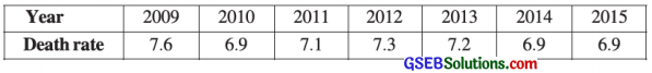
The information about death rate of a state in different years is given in the following table. Fit a linear equation to find trend and hence estimate the death rate for the year 2017.
Answer:
Here, n = 7; So t = 1, 2, …………, 7 and y = Death rate
We fit a linear equation ŷ = a + bt to find trend.
The table to calculate the values of a and b is prepared as follows:
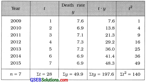
t̄ = \(\frac{\Sigma t}{n}\)
Putting n = 7 and Σt = 28, we get
t̄ = \(\frac{28}{7}\)
= 4
ȳ = \(\frac{\Sigma y}{n}\)
Putting n = 7 and Σy = 49.9, we get
ȳ = \(\frac{49.9}{7}\)
= 7.13
Now, b = \(\frac{n \Sigma t y-(\Sigma t)(\Sigma y)}{n \Sigma t^{2}-(\Sigma t)^{2}}\)
Putting n = 7, Σty = 197.6, Σt = 28, Σy = 49.9 and Σt2 = 140 in the formula,
b = \(\frac{7(197.6)-(28)(49.9)}{7(140)-(28)^{2}}\)
= \(\frac{1383.2-1397.2}{980-784}\)
= \(\frac{-14}{196}\)
= – 0.07
a = ȳ – bt̄
Putting ȳ = 7.13, b = – 0.07 and t̄ = 4, we get
a = 7.13 – (-0.07) (4)
= 7.13 + 0.28
= 7.41
Equation of Linear trend:
Putting a = 7.41 and b = – 0.07 in ŷ = a + bt,
we get
ŷ = 7.41 – 0.07t
Estimate of death rate for the year 2017:
For the year 2017, corresponding t = 9
Putting t = 9 in ŷ = 7.41 – 0.07, we get
ŷ = 7.41 – 0.07 (9)
= 7.41 – 0.63
= 6.78
Hence, the estimate of death rate for the year 2017 obtained is 6.78.

Question 2.
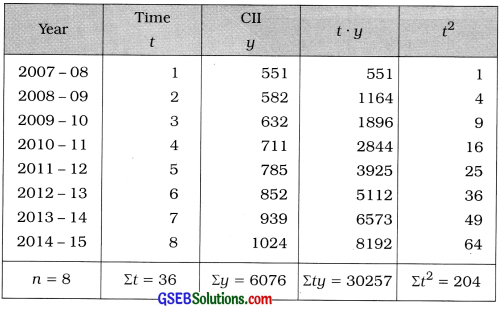
The data about Cost Inflation Index (CII) declared by the central government are as follows. The year 1981 – 82 is the base for this index. Find the estimate of this index for the year 2015-16 by fitting the linear equation to these data.

Answer:
Here, n = 8. So t = 1, 2,…, 8 and y = Cost Inflation Index (CII)
We fit the equation of linear trend ŷ = a + bt
The table for calculating the values of a and b is prepared as follows:
t̄ = \(\frac{\Sigma t}{n}\)
Putting n = 8 and Σt = 36, we get
t̄ = \(\frac{36}{8}\)
= 4.5
ȳ = \(\frac{\Sigma y}{n}\)
Putting n = 8 and Σy = 6076, we get
ȳ = \(\frac{6076}{8}\)
= 759.5
Now, b = \(\frac{n \Sigma t y-(\Sigma t)(\Sigma y)}{n \Sigma t^{2}-(\Sigma t)^{2}}\)
Putting n = 8, Σty = 30257, Σt = 36, Σy = 6076 and Σt2 = 204 in the formula,
b = \(\frac{8(30257)-(36)(6076)}{8(204)-(36)^{2}}\)
= \(\frac{242056-218736}{1632-1296}\)
= \(\frac{23320}{336}\)
= 69.4
a = ȳ – bt̄
Putting ȳ = 759.5, b = 69.4 and t̄ = 4.5, we get
a = 759.5 – 69.4 (4.5)
= 759.5 – 312.3
= 447.2
Equation of linear trend:
Putting a = 447.2 and b = 69.4 in ŷ = a + bt,
we get
ŷ = 447.2 + 69.4t
Estimate of CII for the year 2015-16:
We take t = 9, corresponding to the year 2015-16
Putting t = 9 in ŷ = 447.2 + 69.41, we get
ŷ = 447.2 + 69.4 (9)
= 447.2 + 4 624.6
= 1071.8
Hence, the estimate of CII for the year 2015-16 obtained is 1071.8.
Question 3.
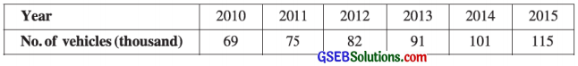
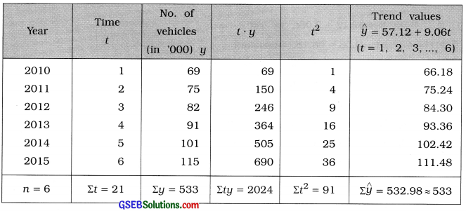
The number of two wheelers registered (in thousand) in a city in different years is as follows. Use the method of fitting linear equation to these data to obtain the estimates for the number of vehicles registered in the year 2016 and 2017. Also find the trend values for each year.
Answer:
Here, n = 6. So t = 1, 2, …………. 6. y = No. of vehicles. We fit the equation of linear trend ŷ = a + bt.
The table to calculate the values of ‘a’ and ‘b’ is prepared as follows:
t̄ = \(\frac{\Sigma t}{n}\)
Putting n = 6 and Σt = 21, we get
t̄ = \(\frac{21}{6}\)
= 3.5
ȳ = \(\frac{\Sigma y}{n}\)
Putting n = 6 and Σy = 533, we get
ȳ = \(\frac{533}{6}\)
= 88.83
Now, b = \(\frac{n \Sigma t y-(\Sigma t)(\Sigma y)}{n \Sigma t^{2}-(\Sigma t)^{2}}\)
Putting n = 6, Σty = 2024, Σt = 21, Σy = 533 and Σt2 = 91 in the formula,
b = \(\frac{6(2024)-(21)(533)}{6(91)-(21)^{2}}\)
= \(\frac{12144-11193}{546-441}\)
= \(\frac{951}{105}\)
= 9.06
a = ȳ – bt̄
Putting ȳ = 88.83, b = 9.06 and t̄ = 3.5, we get
a = 88.83 – 9.06 (3.5)
= 88.83 – 31.71
= 57.12
Equation of linear trend:
Putting a = 57.12 and b = 9.06 in ŷ = a + bt,
we get
ŷ = 57.12 + 9.061.
Estimate for the number of vehicles registered for the year 2016:
We take t = 7, corresponding to the year 2016.
Putting t = 7, in ŷ = 57.12 + 9.06t, we get
ŷ = 57.12 + 9.06 (7)
= 57.12 + 63.42
= 120.54 (thousand)
Hence, the estimate for the number of vehicles registered for the year 2016 obtained is 120.54 thousand.
Estimate for the number of vehicles registered for the year 2017:
We take t = 8, corresponding to the year 2017.
Putting t = 8 in ŷ = 57.12 + 9.061, we get
ŷ = 57.12 + 9.06 (8)
= 57.12 + 72.48
= 129.6 (thousand)
Hence, the estimate for the number of vehicles registered in the year 2017 obtained is 129.6 thousand vehicles.
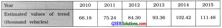
Trend Values :
Putting t=l, 2, …, 6 in ŷ = 57.12 + 9.06t, we get
ŷ = 57.12 + 9.06 (1) = 57.12 + 9.06 = 66.18, (thousand)
= 57.12 + 9.06 (2) = 57.12 + 18.12 = 75.24, (thousand)
= 57.12 + 9.06 (3) = 57.12 + 27.18 = 86.30, (thousand)
= 57.12 + 9.06 (4) = 57.12 + 36.24 = 93.36, (thousand)
= 57.12 + 9.06 (5) = 57.12 + 45.30 = 102.42, (thousand)
= 57.12 + 9.06 (6) = 57.12 + 54.36 = 111.48, (thousand)
Trend values for each year is tabulate as follows:
Question 4.
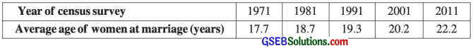
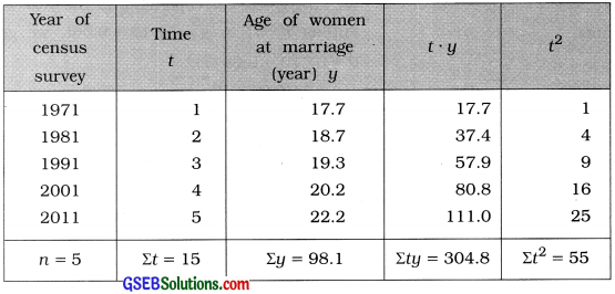
The average age of women (in years) at the time of marriage obtained from the data of different census surveys in India are given in the following table. Fit an equation for a linear trend from the data and show it on a graph. Find the estimate for the value of the given variable for the year 2021 using the linear equation.
Answer:
Here, n = 5. t = \(\frac{\text { Year }-1961}{10}\). So t = 1, 2, …, 5. y = Average age of women at marriage date.
We fit the equation of linear trend ŷ = a + bt.
To calculate the values of ‘a’ and ‘b’ the table prepared as follows:
t̄ = \(\frac{\Sigma t}{n}\)
Putting n = 5 and Σt = 15, we get
t̄ = \(\frac{15}{5}\)
= 3
ȳ = \(\frac{\Sigma y}{n}\)
Putting n = 5 and Σy = 98.1, we get
ȳ = \(\frac{98.1}{5}\)
= 19.62
Now, b = \(\frac{n \Sigma t y-(\Sigma t)(\Sigma y)}{n \Sigma t^{2}-(\Sigma t)^{2}}\)
Putting n = 5, Σty = 304.8, Σt = 15, Σy = 98.1 and Σt2 = 55 in the formula.
b = \(\frac{5(304.8)-(15)(98.1)}{5(55)-(15)^{2}}\)
= \(\frac{1524-1471.5}{275-225}\)
= \(\frac{52.5}{50}\)
= 1.05
a = ȳ – bt̄
Putting ȳ = 19.62, b = 1.05 and t̄ = 3, we get
a = 19.62 – 1.05 (3)
= 19.62 – 3.15
= 16.47
Equation of linear trend:
Putting a = 16.47 and b = 1.05 in ŷ = a + bt,
we get
ŷ = 16.47 + 1.05t
Estimate of average age of women at marriage for the year 2021 :
We take t = 6, corresponding to the year 2021.
Putting t = 6 in ŷ = 16.47 + 1.05t, we get
ŷ = 16.47 + 1.05 (6)
= 16.47 + 6.30
= 22.77 (year)
Graphical representation:
Taking t on X-axis and y on Y-axis points (1, 17.7), (2, 18.7), (3, 19.3), (4, 20.2) and (5, 22) are plotted on the graph paper. Joining these points serially by line, the curve for the given time series is obtained as follows:
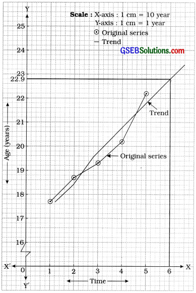
The curve passing through close to most of the points of the curve of original series is the curve showing the trend of the given series. It is clear from the trend curve, that when t = 6, the estimate of average age of women at marriage obtained is approximately 22.9 year.